Use the Xenium Pipeline
 | Abbreviations Key | ||||
| AnnData | annotated data [Python/R package for storing spatial matrices] | MEX | market exchange [format] | ||
| CSV | comma-separated values | MIP | maximum-intensity projection | ||
| FFPE | formalin-fixed paraffin-embedded [tissue preservation method] | OME | open microscopy environment | ||
| gz | gzipped | PCA | principal component analysis | ||
| H5AD | .h5 AnnData [format] | QC | principal component analysis | ||
| HDF5 | Hierarchical Data Format, version 5 [proprietary file format] | scRNA-seq | single-cell RNA sequencing | ||
| H&E/IF | hematoxylin and eosin immunofluorescence [images] | STalign | spatial transcriptomics alignment | ||
| HISE | Human Immune System Explorer | UMAP | uniform manifold approximation and projection | ||
| IDE | integrated development environment | VM | virtual machine | ||
| ISD | instrument sensor data |
At a Glance
The Xenium pipeline enables spatial transcriptomics analysis within HISE, converting raw Xenium data into formats that can be analyzed, explored, and visualized in HISE.
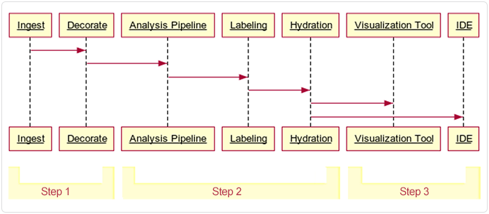
This document describes the pipeline in three broad stages or steps, summarized in Table 1 and depicted in the following image.
| TABLE 1 | ||
| Step | Description | Locations |
| Step 1: Preprocessing | Raw output from the Xenium instrument is preprocessed, quality checked, labeled with spatial and cell type data, and summarized. Some of this data is archived, and the remaining data is prepared for ingestion into HISE. | Output on Xenium, preprocessed on a VM or workstation, and uploaded to cloud storage |
| Step 2: Ingestion | Data is ingested into HISE, where it is further decorated (associated with metadata), analyzed, labeled, and made available for downstream analysis | HISE Project Store (cloud storage and metadata management) |
| Step 3: Exploration | Data is explored, visualized, and further analyzed using advanced search queries, integration with other datasets or data types, and custom plots, such as spatial maps or dimensionality reduction visualizations | HISE NextGen IDE (Jupyter Notebook environment) |
 Preprocessing
It's beyond the scope of this document to cover all of the preprocessing functions in detail, but let's briefly explore how Xenium handles data during this stage. For each FFPE tissue sample, Xenium generates two forms of raw data:
- Initial raw data. First, the 10x machine generates a massive amount of raw ISD data. One Xenium slide with the entire imageable area selected produces its own directory ranging from 7–60 GB, depending on the tissue and the panel. A single run typically contains four slides, for a total of 28-240 GB. (For examples of public datasets, see the 10x Genomics website.) The raw Xenium output files are listed in Table 2.
| TABLE 2 | |||
| File description | File type | File size | Example file name |
| Web summary | HTML | 14,834 KB | analysis_summary.html |
| Gene expression metrics | CSV | 1 KB | metrics_summary.csv |
| Cell-feature matrix | MEX HDF5 Zarr (zipped) | H5: 46,887 KB Zarr: 67,433 KB | cell_feature_matrix.h5 cell_feature_matrix.zarr.zip |
| Transcript data | CSV (gzipped) Parquet Zarr (zipped) | CSV: 3,985,959 KB Parquet: 1,868,732 KB Zarr: 2,477,239 KB | transcripts.csv.gz transcripts.parquet |
| Cell summary file | CSV (zipped) Parquet Zarr (zipped) | CSV: 39,067 KB Parquet: 16,840 KB Zarr: 1,756,885 KB | cells.csv.gz |
| Panel file | JSON | 137 KB | gene_panel.json |
| Morphology | OME-TIF | 33,080,064 KB | morphology.ome.tif morphology_focus.ome.tif morphology_mip.ome.tif |
| Secondary analysis results | CSV Zarr (zipped) | Zarr: 8,136 KB | metrics_summary.csv |
| Cell and nucleus segmentation files | Zarr (zipped) CSV (zipped) Parquet | Zarr: 20,893 KB CSV: 108,623 KB | cell_boundaries.csv.gz nucleus_boundaries.csv.gz nucleus_boundaries.parquet |
| Xenium experiment file | JSON | 2 KB | experiment.xenium |
2. Preprocessed raw data. The machine then parses the data in a smaller raw data set that contains decoded transcript information. This transient data remains active only until cell segmentation, at which point it's also archived. A directory containing the resulting machine-processed data is created. The Xenium preprocessing output directory includes the files listed in Table 3.
| TABLE 3 | ||
| Stage | Output | Example |
| Preprocessing | xenium_<tissue>_adata_filtered.h5ad | Not pictured |
| QC | PDF reports (for example, nucleus/cell area plots) | 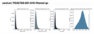 |
| Cell labeling | Cell-type predictions | 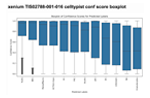 |
| Neighborhood analysis | Spatial cluster plots created using CellCharter | 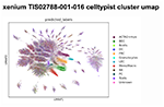 |
| Summary report | <tissue>_pipeline_summary.html | 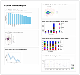 |
 Ingestion
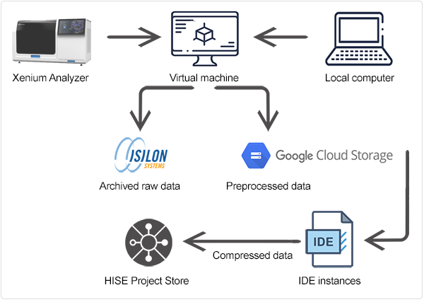
This is where HISE enters the picture. The necessary configuration files are ingested (Table 4). Then the preprocessed Xenium files (see Table 3) are moved into a watchfolder, which triggers ingestion of the data into HISE. (Be sure to follow this sequence, since the pipeline run will fail if the tar file is ingested before the configuration files.)
| TABLE 4 | |
| Config file | Description |
| xenium_pipeline_config-colon.json | Colon tissue-specific parameters |
| xenium_pipeline_config-default.json | Default settings for all tissues |
| xenium_pipeline_config-ln.json | Lymph node-specific parameters |
| xenium_pipeline_config-tonsil.json | Tonsil tissue-specific parameters |
The data ingestion workflow, including preprocessing, is shown in the accompanying figure.
During ingest, the directory is unzipped into /processed_data/. The files in this new directory are listed in Table 5.
| TABLE 5 | |||
| File type | Example file name | Content | Purpose |
| Binary HDF5 file | cell_feature_matrix.h5 | Cell-by-gene expression matrix | Serves as the primary quantitative input for downstream analysis and AnnData conversion |
| CSV (zipped) | cells.csv.gz | Cell-level metadata | Supplies QC info for each cell |
| Zarr (zipped) | cells.zarr.zip | Segmentation masks and boundaries for cells and nuclei | Used for spatial mapping, cell segmentation, and morphology analysis |
| CSV | metrics_summary.csv | Run-level and sample-level metrics | Used to assess run quality and to fetch sample/region IDs for pipeline processing |
TIF or OME-TIF | Xenium_FFPE_Human_Breast_Cancer_Rep1_he_image.tif GSM7780153_Post-Xenium_HE_Rep1.ome.tif | Post-Xenium H&E/IF images | Visualization and spatial context |
Unlike other types of data, Xenium data doesn't require a sample or submission sheet. You can simply ingest the raw data into HISE, which handles organization, validation, and metadata extraction for you. A filename looks something like this:
202208311221_EXP-00422-LN-FFPE-NDGFKF_XETG00123_region_A1
Output of results
Table 6 contains a list of downloadable/servable result file types.
| TABLE 6 | |||||||
| File Type | Kind | Name | File Type | Kind | Name | ||
| control-xenium-tar-content | Wildcard | Control Xenium Tar Content | xenium-filtered-h5ad | H5 | Xenium Filtered H5ad | ||
| scvi-model | .PT | SCVI Model | xenium-filtered-qc-pdf | filtered_qc.pdf | |||
| xenium-10-x-report | HTML | Xenium 10X Report | xenium-gene-panel-json | JSON | Xenium Gene Panel Json | ||
| xenium-analysis-zarr | Zarr | Xenium Analysis Zarr | xenium-h5ad | H5 | Xenium H5ad | ||
| xenium-cell-boundaries-csv | CSV-GZ | Xenium Cell Boundaries CSV | xenium-metrics-summary-csv | CSV | Xenium Metrics Summary CSV | ||
| xenium-cell-boundaries-parquet | Parquet | Xenium Cell Boundaries Parquet | xenium-morphology-0-tif | TIF | Xenium Morphology 0 Tif | ||
| xenium-cell-composition-counts-csv | CSV | Xenium Cell Composition Counts Csv | xenium-morphology-1-tif | TIF | Xenium Morphology 1 Tif | ||
| xenium-cell-composition-fractions-csv | CSV | Xenium Cell Composition Fractions Csv | xenium-morphology-2-tif | TIF | Xenium Morphology 2 Tif | ||
| xenium-cell-feature-h5 | H5 | Xenium Cell Feature H5 | xenium-morphology-3-tif | TIF | Xenium Morphology 3 Tif | ||
| xenium-cell-feature-zarr | Zarr.Zip | Xenium Cell Feature Zarr | xenium-morphology-ome-tif | TIF | Xenium Morphology OME TIF | ||
| xenium-cellcharter-cluster-pdf | Xenium Cellcharter Cluster Pdf | xenium-nucleus-boundaries-csv | CSV | Xenium Nucleus Boundaries CSV | |||
| xenium-cellcharter-h5ad | H5 | Xenium Cellcharter H5ad | xenium-nucleus-boundaries-parquet | Parquet | Xenium Nucleus Boundaries Parquet | ||
| xenium-cellcharter-predictions-joblib | JobLib | Xenium Cellcharter Predictions Joblib | xenium-qc-filtered-h5ad | H5 | Xenium QC Filtered H5ad | ||
| xenium-cellcharter-stability-plot-pdf | Xenium Cellcharter Stability Plot Pdf | xenium-qc-pdf | Xenium QC PDF | ||||
| xenium-cells-csv | CSV | Xenium Cells Csv | xenium-raw-qc-pdf | Xenium Raw QC Pdf | |||
| xenium-cells-parquet | Parquet | Xenium Cells Parquet | xenium-tar-content | Wildcard | Xenium Tar Content | ||
| xenium-cells-zarr | Zarr | Xenium Cells Zarr | xenium-transcripts-csv | CSV | Xenium Transcripts CSV | ||
| xenium-celltypist-cluster-umap-pdf | Xenium Celltypist Cluster Map Umap Pdf | xenium-transcripts-parquet | Parquet | Xenium Transcripts Parquet | |||
| xenium-celltypist-predicted-labels-csv | CSV | Xenium Celltypist Predicted Labels Csv | xenium-transcripts-zarr | Zarr | Xenium Transcripts Zarr | ||
| xenium-celltypist-predictions-h5ad | H5 | Xenium Celltypist Predictions H5ad | xenium-zone-cell-type-counts-pdf | Xenium Zone Cell Type Counts PDF | |||
| xenium-celltypist-predictions-joblib | JobLib | Xenium Celltypist Predictions Joblib | xenium-zone-cell-type-fractions-csv | CSV | Xenium Zone Cell Type Fractions CSV | ||
| xenium-experiment | .xenium | Xenium Experiment |
Visualization of results
You can use an interactive visualization tool to understand your results. Examples of the types of visualizations you can create are listed in Table 7.
| TABLE 7 | |
| Visualization | Description |
| Spatial maps | Overlay gene expression or cell types on tissue images using |
| Cluster plots | Visualize clusters or cell types in reduced dimensions |
| QC plots | Display metrics like total counts per cell, number of genes per cell, or cell/nucleus area |
| Bar charts, heat maps, or violin plots | Summarize cell composition, gene expression, or spatial domains |
 Exploration
After ingestion, your data is ready for exploration and interactive analysis in a HISE NextGen IDE.
Interactive data analysis
The Jupyter Notebook/IDE environment is used for intersample analysis in either interactive mode (manually interacting with a Jupyter notebook) or batch mode (notebook jobs). You can load AnnData (.h5ad) files and other outputs for custom analysis using Python libraries such as Scanpy, Squidpy, or Seaborn. You can also perform dimensionality reduction (for example, UMAP, t-SNE, or PCA) and clustering. Another option is to run an advanced query to filter cells by type, spatial region, or gene expression.
For deeper biological insights, you can combine Xenium data with other spatial transcriptomics datasets, such as Visium, or with scRNA-seq data. For cross-dataset analysis, batch correction, or spatial alignment, you can integrate tools like Scanpy, Squidpy, or STalign. Then export your results for further downstream analysis or publication.
 Related Resources
Submit and Monitor Pipeline Batches (Tutorial)