Overview
To allow scientists to label their own PBMC datasets using the labels defined in our Human Immune Health Atlas, we provide models for CellTypist at each level of resolution.
View Notebook: Python_AIFI_CellTypist_labeling.ipynb
AIFI_L1: 9 broad cell classes
AIFI_L2: 29 major cell types
AIFI_L3: 71 high-resolution cell types
These models can be obtained from the Downloads page. More information about CellTypist can be found in Domínguez Conde, et al. (2022) and at https://www.celltypist.org/.
For comparison to our CellTypist models, we'll also label cells with a model provided by the CellTypist website generated from data provided in Stephenson, et al. (2021).
Demonstration
To demonstrate how to label your own data using our model, we'll label a PBMC dataset previously published in Swanson, et al. (2022) and available at GEO Accession GSM5513397.
This demonstration is written in Python, as CellTypist is available as a Python module. We also utilize the Scanpy package for single-cell data analysis, described in Wolf, et al. (2018).
Install Packages
!pip install -q scanpy
!pip install -q celltypist
!pip install -q session_info
Load Modules
from urllib.request import urlretrieve

import celltypist
import scanpy as sc
Specify CellTypist models
In addition to our own CellTypist models, we'll use a Healthy PBMC model provided from the CellTypist model collection:
celltypist.models.download_models(
    force_update = True,
    model = ['Healthy_COVID19_PBMC.pkl']
)
Here, we specify the path to the CellTypist models. For this demo, we assume the AIFI CellTypist models have been downloaded from the Downloads Page, and are placed in the working directory.
model_files = {
    'CellTypist_PBMC': 'Healthy_COVID19_PBMC.pkl',
    'AIFI_L1': 'ref_pbmc_clean_celltypist_model_AIFI_L1_2024-04-18.pkl',
    'AIFI_L2': 'ref_pbmc_clean_celltypist_model_AIFI_L2_2024-04-19.pkl',
    'AIFI_L3': 'ref_pbmc_clean_celltypist_model_AIFI_L3_2024-04-19.pkl'
}
Download dataset from GEO
Next, we'll download the dataset we want to label from GEO. This .h5 file is provided as a Supplementary File in the GEO entry for GSM5513397
geo_url = "https://www.ncbi.nlm.nih.gov/geo/download/?acc=GSM5513397&format=file&file=GSM5513397%5FW4%2Dhashed%2D24k%5Fcount%2Dmatrix%2Eh5"
h5_filename = "GSM5513397_W4-hashed-24k_count-matrix.h5"
urlretrieve(geo_url, h5_filename)
Load and normalize data with Scanpy
Next, we'll load the dataset using Scanpy, and normalize and log transform the data to meet the requirements of the CellTypist module for labeling.
adata = sc.read_10x_h5(h5_filename)
adata
AnnData object with n_obs × n_vars = 14478 × 36601
var: 'gene_ids', 'feature_types', 'genome'sc.pp.normalize_total(adata, target_sum = 1e4)
sc.pp.log1p(adata)Predict labels with each model
Now, we can loop through each model specified above and label the cells using CellTypist.
CellTypist provides multiple kinds of results about these labels. For this demo, we'll keep just the highest scoring label and the corresponding labeling score generated by CellTypist.
label_results = {}

for model_name, model in model_files.items():
    label_column = f'{model_name}_prediction'
    score_column = f'{model_name}_score'

    predictions = celltypist.annotate(
        adata,
        model = model
    )

    labels = predictions.predicted_labels
    labels = labels.rename({'predicted_labels': label_column}, axis = 1)

    prob = predictions.probability_matrix
    prob_scores = []
    for i in range(labels.shape[0]):
        prob_scores.append(prob.loc[labels.index.to_list()[i],labels[label_column][i]])
    labels[score_column] = prob_scores

    label_results[model_name] = labels
Preview results for each model
After generating label predictions, let's look at the top 10 labels assigned by each of the labeling models:
for model_name, label_df in label_results.items():
    label_column = f'{model_name}_prediction'
    label_summary = label_df[label_column].value_counts()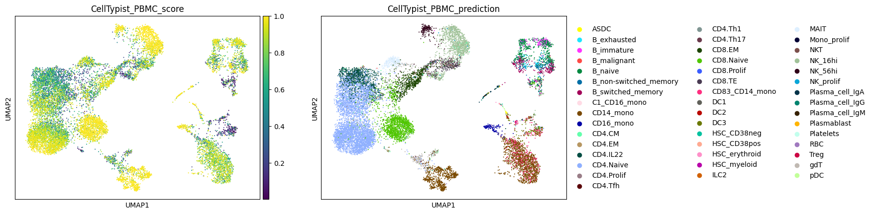
print(label_summary[0:10], end = '\n\n')CellTypist_PBMC_prediction
CD4.Naive 4661
CD14_mono 1976
CD8.Naive 1614
NK_16hi 1184
CD4.IL22 949
CD8.EM 615
B_naive 580
MAIT 432
CD83_CD14_mono 387
gdT 312
Name: count, dtype: int64
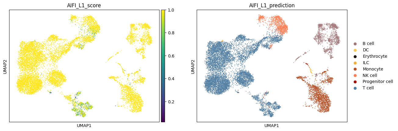
AIFI_L1_prediction
T cell 9955
Monocyte 1902
B cell 1423
NK cell 1119
DC 45
Progenitor cell 22
ILC 10
Erythrocyte 2
Name: count, dtype: int64
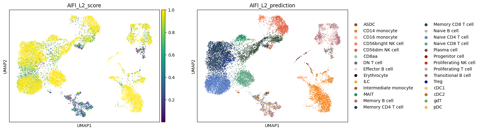
AIFI_L2_prediction
Memory CD4 T cell 3099
Naive CD4 T cell 2733
CD14 monocyte 2010
Naive CD8 T cell 1486
Memory CD8 T cell 1320
CD56dim NK cell 1009
Naive B cell 685
Memory B cell 557
MAIT 339
Treg 270
Name: count, dtype: int64
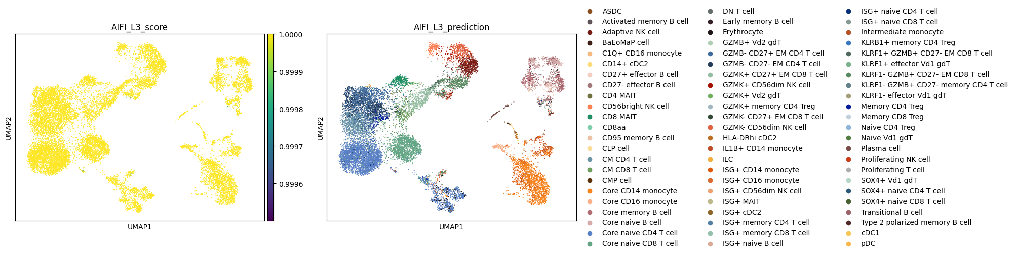
AIFI_L3_prediction
Core naive CD4 T cell 3112
Core naive CD8 T cell 1443
Core CD14 monocyte 1377
GZMB- CD27+ EM CD4 T cell 1326
CM CD4 T cell 888
GZMB- CD27- EM CD4 T cell 741
Adaptive NK cell 587
GZMK+ CD27+ EM CD8 T cell 467
KLRF1- GZMB+ CD27- EM CD8 T cell 444
Core memory B cell 433
Name: count, dtype: int64Add labels to the dataset
In order to use the labels for visualization, as well as any downstream analyses we might want to do, we'll add the labels and scores from our celltypist labels to the AnnData object.
for model_name, label_df in label_results.items():
    label_column = f'{model_name}_prediction'
    score_column = f'{model_name}_score'

    adata.obs[label_column] = label_df[label_column]
    adata.obs[score_column] = label_df[score_column]
Dimensionality reduction for visualization
Next, we can perform dimensionality reduction with PCA and 2-dimensional projection with UMAP to allow us to visualize the labels on the data.
sc.pp.highly_variable_genes(adata)
sc.tl.pca(adata)
sc.pp.neighbors(adata, n_pcs = 30)
sc.tl.umap(adata)
Optional: Add colorsets for visualization
If you want to match the colors used in our publications, you can do so by reading the colorset tables we provide on our Downloads page.
color_files = {
    'AIFI_L1': 'AIFI_L1_imm_health_atlas_type_order_colors.csv',
    'AIFI_L2': 'AIFI_L2_imm_health_atlas_type_order_colors.csv',
    'AIFI_L3': 'AIFI_L3_imm_health_atlas_type_order_colors.csv'
}
Generate dictionaries for matching colors to categorical value order
color_dicts = {}
for level, file in color_files.items():
    color_df = pd.read_csv(file)
    color_dict = {}
    for i in range(color_df.shape[0]):
        cell_type = color_df[level].loc[i]
        type_color = color_df[f'{level}_color'].loc[i]
        color_dict[cell_type] = type_color
    color_dicts[level] = color_dict
Assign colors to the AnnData object
for level, color_dict in color_dicts.items():
    color_order = adata.obs[f'{level}_prediction'].cat.categories
    level_colors = [color_dict[x] for x in color_order]
    adata.uns[f'{level}_prediction_colors'] = level_colors
Plot labels on UMAP projections
Finally, let's plot the labeling scores and cell type labels from each CellTypist model.
Note: Due to the use of a multinomial regression for training of the AIFI_L3 model, the AIFI_L3_score values are higher than those for the other models.
for model_name in label_results.keys():
    label_column = f'{model_name}_prediction'
    score_column = f'{model_name}_score'

    sc.pl.umap(
        adata,
        color = [score_column, label_column]
    )
Save labeled data
For later analysis, we can save the labeled dataset to disk as a .h5ad file.
adata.write_h5ad('labeled_GSM5513397_W4-hashed-24k_count-matrix.h5')Session Information
Below are details of the versions of Python and the Python Modules used for this demonstration.
import session_info
session_info.show()-----
anndata 0.10.3
celltypist 1.6.3
pandas 2.1.4
scanpy 1.9.6
session_info 1.0.0
-----
Click to view modules imported as dependencies
-----
IPython 8.19.0
jupyter_client 8.6.0
jupyter_core 5.6.1
jupyterlab 4.1.5
notebook 6.5.4
-----
Python 3.10.13 | packaged by conda-forge | (main, Dec 23 2023, 15:36:39) [GCC 12.3.0]
Linux-5.15.0-1062-gcp-x86_64-with-glibc2.31
-----
Session information updated at 2024-07-15 01:35References
Domínguez Conde C, Xu C, Jarvis LB, Rainbow DB, Wells SB, Gomes T, et al. Cross-tissue immune cell analysis reveals tissue-specific features in humans. Science. 2022;376: eabl5197.
doi:10.1126/science.abl5197
Stephenson E, Reynolds G, Botting RA, Calero-Nieto FJ, Morgan MD, Tuong ZK, et al. Single-cell multi-omics analysis of the immune response in COVID-19. Nat Med. 2021;27: 904–916.
doi:10.1038/s41591-021-01329-2
Swanson E, Reading J, Graybuck LT, Skene PJ. BarWare: efficient software tools for barcoded single-cell genomics. BMC Bioinformatics. 2022;23: 106.
doi:10.1186/s12859-022-04620-2
Wolf FA, Angerer P, Theis FJ. SCANPY: large-scale single-cell gene expression data analysis. Genome Biol. 2018;19: 15.
doi:10.1186/s13059-017-1382-0